Orbit Determination Workflow

This workflow reproduces the 2025 BC10 orbit-determination validation case included with DiffOrb. It fits a mixed optical and radar observation set, checks station-level residual statistics, changes one station from the default optical weights to reported ADES uncertainties, and compares the final orbit with the JPL Horizons JPL#51 solution.

The final product is a fitted BCRS Cartesian state at JD 2460762.5 TDB, its covariance, residual diagnostics, and a one-year optical prediction check.

Prerequisites

• Activate the project environment described in Installation.
• Use a planetary kernel such as de441.bsp.
• Use the SB441-N16 asteroid-perturber kernel.
• Use online access to fetch fresh MPC and JPL observations, or use a local ADES PSV cache.
• Install astroquery and use online access when you run the Horizons comparison code.
• Treat the printed values below as reference output for the bundled validation data. Online observation data can change.

For the model behind the solve, read Orbit Determination Overview, Initial Orbit Determination, Differential Correction, Weighting And Debiasing Models, and Outlier Rejection.

Load Data

2025 BC10 was discovered by Pan-STARRS 1 on 2025-01-28. It made a close Earth approach in early April 2025, when Goldstone radar delay and Doppler observations were obtained. The validation case uses 799 optical observations from the IAU MPC and 8 radar observations from the JPL Small-Body Radar Astrometry database.

Load the ephemeris first. Then load the observation set. Use load_online_observations(...) when you want to refresh the data. Use load_local_observations(...) when you want a fixed cached PSV file.

from pathlib import Path

from difforb.astrometry import load_local_observations, load_online_observations
from difforb.spk import Ephemeris, set_default_ephemeris

planetary_kernel = Path("/path/to/de441.bsp")
asteroid_kernel = Path("/path/to/sb441-n16.bsp")
observation_cache = Path("cache/2025_BC10-online.psv")

ephemeris = Ephemeris([str(planetary_kernel), str(asteroid_kernel)])
set_default_ephemeris(ephemeris)

if observation_cache.exists():
    obs = load_local_observations(str(observation_cache))
else:
    obs = load_online_observations("2025 BC10", save_path=str(observation_cache))

print("NAME", obs.name)
print("N_OBS", len(obs))
print("N_OPTICAL", obs.num_optical)
print("N_RADAR", obs.num_radar)
print("T_START", obs.t_start.ut.iso_string)
print("T_END", obs.t_end.ut.iso_string)

Reference output

NAME 2025 BC10
N_OBS 807
N_OPTICAL 799
N_RADAR 8
T_START 2025-01-28 13:31:33.500
T_END 2025-04-06 06:39:50.960

Build The Model

Use the extended dynamical system. It uses the planetary background and the supported asteroid perturbers. Use IAS15 for the integration.

from difforb.body import EphemerisBody
from difforb.dynamics import DynamicSystem
from difforb.integrator import NumericalIntegrator
from difforb.od import DCBucketPolicy, DCSolver, IODSolver, ODSolver

force_model = DynamicSystem.from_extended_system(ephemeris).build_force_model()
integrator = NumericalIntegrator(
    method="IAS15",
    tol=1e-12,
    max_steps=4096,
    initial_step=1e-6,
)

solver = ODSolver(
    IODSolver(),
    DCSolver(
        lsq_tol=1e-11,
        lsq_max_iters=20,
        sun=EphemerisBody("sun", eph=ephemeris),
        earth=EphemerisBody("earth", eph=ephemeris),
        bucket_policy=DCBucketPolicy(),
    ),
)

This sets the force and integration path used for the 2025 BC10 validation case. The target small body is integrated. The Sun, planets, Moon, Pluto, and asteroid perturbers are read from SPK ephemerides.

Configure The Solve

The initial orbit uses a 1 day optical arc. Differential correction then uses the full observation arc in one stage. The optical baseline is the VFCC17 weighting model with EgglDebiasPolicy. Radar rows use their reported uncertainties. The chi-square outlier rejection thresholds are tighter than the defaults.

from difforb.astrometry import ADESWeightPolicy, EgglDebiasPolicy, InteractiveWeightPolicy, VFCC17WeightPolicy
from difforb.od import Chi2OutlierRejecter, DCStrategy, IODStrategy, InteractiveOutlierPolicy

iod_strategy = IODStrategy(
    arc_days=1.0,
    max_candidates=10,
    init_rho=(1.0, 1.0),
)

dc_strategy = DCStrategy(
    incremental_arc_days=[1.0e9],
    min_observations=3,
    epoch_strategy="keep_initial",
)

vfcc = VFCC17WeightPolicy()
ades = ADESWeightPolicy()
debias_policy = EgglDebiasPolicy()


def make_outlier_policy():
    return InteractiveOutlierPolicy(
        Chi2OutlierRejecter(
            chi2_rej_2d=3.5,
            chi2_rec_2d=2.5,
        ),
        enable_auto_rejecter=True,
        max_iters=10,
    )

The make_outlier_policy() helper returns a fresh policy for each solve. This keeps the first and second solves independent.

Run The Baseline Solve

Run the first solve with VFCC17WeightPolicy for optical observations. Then inspect station-level normalized residual spread.

from difforb.od import ODAnalysis

first_weight_policy = InteractiveWeightPolicy(
    default_policy=vfcc,
    additional_policies=[ades],
)

first_result = solver.solve(
    obs,
    force_model=force_model,
    integrator=integrator,
    weight_policy=first_weight_policy,
    debias_policy=debias_policy,
    outlier_policy=make_outlier_policy(),
    iod_strategy=iod_strategy,
    dc_strategy=dc_strategy,
    log_detail="quiet",
)

first_dc = first_result.dc_result
first_analysis = ODAnalysis.from_result(obs, first_dc)
first_stats = first_analysis.station_summary()

cols = [
    "station_key",
    "obs",
    "inliers",
    "normalized_residual_spread",
    "std_normalized_ra_residual",
    "std_normalized_dec_residual",
]

w74_first = first_stats[first_stats["station_key"] == "W74"]

print("FIRST_NORMALIZED_RESIDUAL_RMS", f"{first_dc.normalized_residual_rms:.6f}")
print("FIRST_OPTICAL_INLIERS", first_dc.optical.n_inliers, first_dc.optical.n_obs)
print("FIRST_RADAR_INLIERS", first_dc.radar.n_inliers, first_dc.radar.n_obs)
print(w74_first[cols].to_string(index=False))

Reference output

FIRST_NORMALIZED_RESIDUAL_RMS 0.265859
FIRST_OPTICAL_INLIERS 791 799
FIRST_RADAR_INLIERS 8 8
station_key  obs  inliers  normalized_residual_spread  std_normalized_ra_residual  std_normalized_dec_residual
        W74   22       22                    0.048865                    0.045909                    0.051652

The normalized residual spread is the standard deviation of residuals after division by the adopted uncertainties. A value near 1 is expected when the adopted uncertainties match the residual scatter. Station W74 has 22 optical observations and a spread near 0.049, so the default VFCC17 uncertainty for this station is conservative for this arc.

Use ADES Weights For W74

The ADES data for W74 include reported optical uncertainties. Use those reported uncertainties only for W74, then run the same orbit-determination path again.

import numpy as np

optical = obs.optical
station_codes = np.asarray(optical.rx_codes)
override_indices = optical[station_codes == "W74"].input_indices

final_weight_policy = InteractiveWeightPolicy(
    default_policy=vfcc,
    additional_policies=[ades],
)
final_weight_policy.select_scheme(override_indices, ades)

final_result = solver.solve(
    obs,
    force_model=force_model,
    integrator=integrator,
    weight_policy=final_weight_policy,
    debias_policy=debias_policy,
    outlier_policy=make_outlier_policy(),
    iod_strategy=iod_strategy,
    dc_strategy=dc_strategy,
    log_detail="quiet",
)

final_dc = final_result.dc_result
final_analysis = ODAnalysis.from_result(obs, final_dc)
final_stats = final_analysis.station_summary()
w74_final = final_stats[final_stats["station_key"] == "W74"]

print("OVERRIDE_COUNT", len(override_indices))
print("FINAL_NORMALIZED_RESIDUAL_RMS", f"{final_dc.normalized_residual_rms:.6f}")
print("FINAL_OPTICAL_INLIERS", final_dc.optical.n_inliers, final_dc.optical.n_obs)
print("FINAL_RADAR_INLIERS", final_dc.radar.n_inliers, final_dc.radar.n_obs)
print(w74_final[cols].to_string(index=False))

Reference output

OVERRIDE_COUNT 22
FINAL_NORMALIZED_RESIDUAL_RMS 0.285276
FINAL_OPTICAL_INLIERS 783 799
FINAL_RADAR_INLIERS 8 8
station_key  obs  inliers  normalized_residual_spread  std_normalized_ra_residual  std_normalized_dec_residual
        W74   22       14                    0.729107                    0.839756                    0.598334

The final normalized residual RMS is larger because the W74 uncertainty is smaller and the normalized residuals are therefore stricter. The W74 spread moves much closer to 1. The radar rows remain in the fit.

Inspect The Final State

The final DCResult stores the fitted orbit and covariance. The state is in BCRS at JD 2460762.5 TDB.

orbit = final_dc.estimate.orbit
unc = final_dc.estimate.uncertainties

def sci(value):
    return f"{float(value): .15E}"

print("EPOCH_TDB_JD", f"{float(orbit.tdb.jd):.9f}")
print("FINAL_STATE_BCRS_AU_AU_PER_D")
print(f"X ={sci(orbit.pos[0])} Y ={sci(orbit.pos[1])} Z ={sci(orbit.pos[2])}")
print(f"VX={sci(orbit.vel[0])} VY={sci(orbit.vel[1])} VZ={sci(orbit.vel[2])}")

Reference output

EPOCH_TDB_JD 2460762.500000000
FINAL_STATE_BCRS_AU_AU_PER_D
X =-1.108504390971626E+00 Y =-1.355488149626378E-01 Z =-3.950206056856146E-02
VX= 1.471064092128955E-02 VY=-1.150860841217882E-02 VZ=-6.603141625273408E-03

Component	Value	1-sigma uncertainty
x (au)	-1.108504390971626E+00	1.504E-08
y (au)	-1.355488149626378E-01	8.104E-09
z (au)	-3.950206056856146E-02	1.062E-08
vx (au / d)	+1.471064092128955E-02	2.082E-09
vy (au / d)	-1.150860841217882E-02	8.382E-10
vz (au / d)	-6.603141625273408E-03	1.033E-09

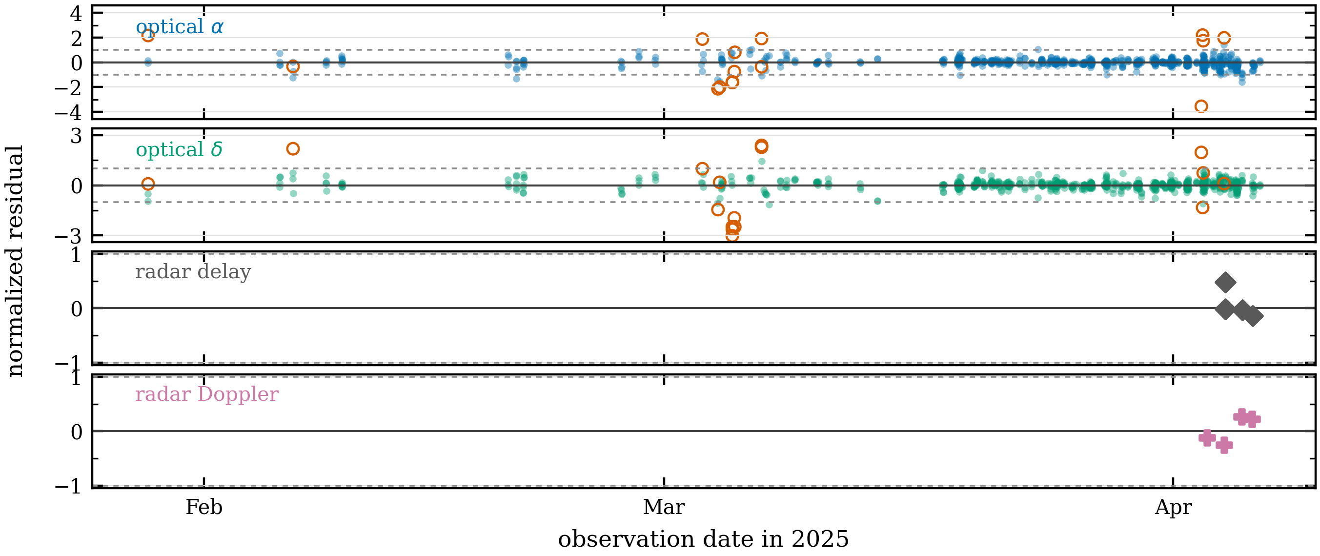
The residual plot below shows the final solution. Filled optical points are retained observations. Open orange circles are rejected optical observations.

Compare With JPL Horizons

As an external check, compare the fitted state with a JPL Horizons state at the same epoch and in the same BCRS state convention. The reference output below is for the JPL#51 solution used by the bundled validation data. A fresh Horizons query can change when JPL updates the small-body solution.

import numpy as np
from astroquery.jplhorizons import Horizons

AU_KM = 149_597_870.700
DAY_S = 86_400.0

orbit = final_dc.estimate.orbit
epoch_tdb_jd = float(orbit.tdb.jd)

horizons_vectors = Horizons(
    id="2025 BC10",
    id_type="smallbody",
    location="@0",
    epochs=epoch_tdb_jd,
).vectors(
    refplane="frame",
    aberrations="geometric",
    cache=True,
)

row = horizons_vectors[0]
jpl_state = np.array(
    [row["x"], row["y"], row["z"], row["vx"], row["vy"], row["vz"]],
    dtype=float,
)
difforb_state = np.concatenate(
    [
        np.asarray(orbit.pos, dtype=float),
        np.asarray(orbit.vel, dtype=float),
    ]
)
delta = difforb_state - jpl_state

print("JPL_STATE")
print(f"X ={jpl_state[0]: .15E} Y ={jpl_state[1]: .15E} Z ={jpl_state[2]: .15E}")
print(f"VX={jpl_state[3]: .15E} VY={jpl_state[4]: .15E} VZ={jpl_state[5]: .15E}")
print("DIFFORB_MINUS_JPL")
print(f"dX  = {delta[0]: .15E} au")
print(f"dY  = {delta[1]: .15E} au")
print(f"dZ  = {delta[2]: .15E} au")
print(f"dVX = {delta[3]: .15E} au / d")
print(f"dVY = {delta[4]: .15E} au / d")
print(f"dVZ = {delta[5]: .15E} au / d")
print(f"|dR| = {np.linalg.norm(delta[:3]):.15E} au")
print(f"|dR| = {np.linalg.norm(delta[:3]) * AU_KM:.3f} km")
print(f"|dV| = {np.linalg.norm(delta[3:]):.15E} au / d")
print(f"|dV| = {np.linalg.norm(delta[3:]) * AU_KM / DAY_S * 1.0e6:.3f} mm / s")

Reference output

JPL_STATE
X =-1.108504391258646E+00 Y =-1.355488131821231E-01 Z =-3.950206028917325E-02
VX= 1.471064088129151E-02 VY=-1.150860827114451E-02 VZ=-6.603142188593907E-03
DIFFORB_MINUS_JPL
dX  = 2.870197413074038E-10 au
dY  =-1.780514707894199E-09 au
dZ  =-2.793882070140086E-10 au
dVX = 3.999803960264003E-11 au / d
dVY =-1.410343074964571E-10 au / d
dVZ = 5.633204996219332E-10 au / d
|dR| = 1.825012527942270E-09 au
|dR| = 0.273 km
|dV| = 5.820829016191457E-10 au / d
|dV| = 1.008 mm / s

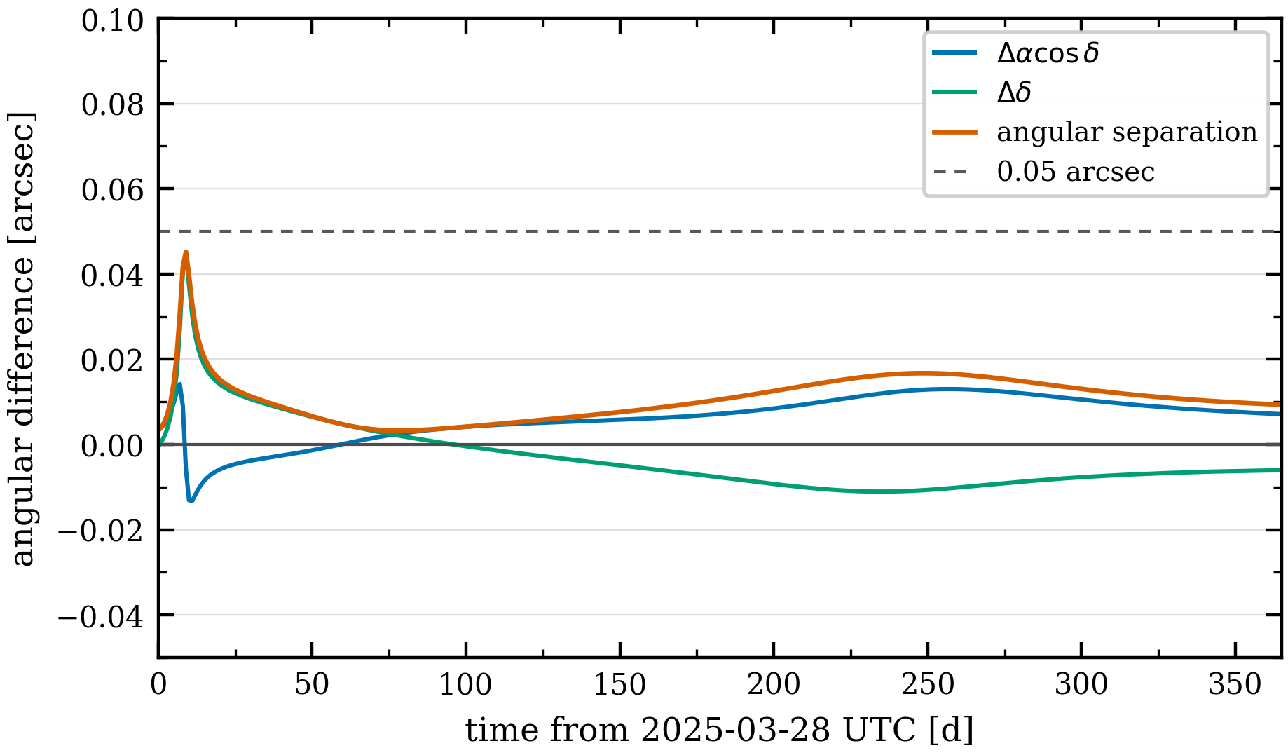
The same fitted state can be propagated for one year and compared with Horizons optical astrometry. This code uses Xinglong station (327) on a daily UTC grid starting on 2025-03-28.

import astropy.units as u
import jax.numpy as jnp
import numpy as np
from astropy.coordinates import SkyCoord
from astroquery.jplhorizons import Horizons

from difforb.body import Site, SmallBody
from difforb.core import Time
from difforb.ephemeris import EphemerisGenerator

observer_code = "327"
offsets_days = np.arange(0.0, 365.0 + 0.5, 1.0, dtype=float)
times = Time.from_utc_date(2025, 3, 28) + jnp.asarray(offsets_days)

target = SmallBody.create(final_dc.estimate.orbit).propagate(
    t_start=Time.from_utc_date(2025, 3, 25).tdb(),
    t_end=Time.from_utc_date(2026, 4, 15).tdb(),
    force_model=force_model,
    integrator=integrator,
)

difforb_table = EphemerisGenerator(target).optical_table(
    times,
    Site.from_code(observer_code),
)
difforb_ra = np.asarray(difforb_table.astrometric_ra, dtype=float)
difforb_dec = np.asarray(difforb_table.astrometric_dec, dtype=float)

horizons_ephem = Horizons(
    id="2025 BC10",
    id_type="smallbody",
    location=observer_code,
    epochs={
        "start": "2025-Mar-28",
        "stop": "2026-Mar-28",
        "step": "1d",
    },
).ephemerides(
    refsystem="ICRF",
    refraction=False,
    extra_precision=True,
    quantities="1",
    cache=True,
)

horizons_ra = np.asarray(horizons_ephem["RA"], dtype=float)
horizons_dec = np.asarray(horizons_ephem["DEC"], dtype=float)

if horizons_ra.shape != difforb_ra.shape:
    raise RuntimeError(f"Horizons returned {horizons_ra.size} epochs; expected {difforb_ra.size}.")

delta_ra_cosdec_arcsec = (
    (difforb_ra - horizons_ra + 180.0) % 360.0 - 180.0
) * np.cos(np.deg2rad(horizons_dec)) * 3600.0
delta_dec_arcsec = (difforb_dec - horizons_dec) * 3600.0

difforb_coord = SkyCoord(ra=difforb_ra * u.deg, dec=difforb_dec * u.deg, frame="icrs")
horizons_coord = SkyCoord(ra=horizons_ra * u.deg, dec=horizons_dec * u.deg, frame="icrs")
separation_arcsec = difforb_coord.separation(horizons_coord).to_value(u.arcsec)

print("MEDIAN_SEPARATION_ARCSEC", f"{np.median(separation_arcsec):.4f}")
print("P95_SEPARATION_ARCSEC", f"{np.percentile(separation_arcsec, 95.0):.4f}")
print("MAX_SEPARATION_ARCSEC", f"{np.max(separation_arcsec):.4f}")

One-year optical prediction comparison

MEDIAN_SEPARATION_ARCSEC 0.0105
P95_SEPARATION_ARCSEC 0.0167
MAX_SEPARATION_ARCSEC 0.0452

The largest separation occurs near the 2025 close approach, where a small Cartesian state difference projects to a larger topocentric sky-plane angle.

Read The Result

The final DCResult is the main product of the workflow.

• final_dc.estimate.orbit is the fitted BCRS state.
• final_dc.estimate.cov_mat_post is the posterior covariance matrix.
• final_dc.normalized_residual_rms is the final normalized residual RMS.
• final_dc.optical and final_dc.radar hold residual blocks and inlier counts.
• ODAnalysis.from_result(obs, final_dc).station_summary() gives station-level residual statistics.
• ODAnalysis.from_result(obs, final_dc).observations gives row-level residuals, chi-square metrics, and inlier flags.

The state comparison with JPL#51 and the one-year optical prediction comparison are external checks. They do not replace residual checks, outlier review, covariance checks, or station-level residual inspection.