Ephemeris Products Workflow

This workflow starts from one fixed orbit for 85472 Xizezong. It propagates the orbit once. It then uses the same propagated trajectory to make optical, vector, radar, element, and event products.

The last section compares the optical output with JPL Horizons for one target and for a random set of numbered small bodies.

Prerequisites

• Activate the project environment described in Installation.
• Use a planetary SPK kernel such as DE441.
• Use a small-body SPK kernel such as SB441-N16.
• Make Earth orientation data available through difforb.core.eop.
• For the Horizons comparison, install astroquery, astropy, numpy, matplotlib, and tqdm.
• For the Horizons comparison, allow network access to JPL Horizons.

This workflow uses DE441 for planets and the Moon. It uses SB441-N16 for the 16 small-body perturbers used by DynamicSystem.from_extended_system().

Build And Propagate The Target

Use the fixed BCRS state below as the starting orbit. The state comes from JPL Horizons at 2461000.5 TDB, which Horizons labels as 2025-Nov-21.0.

The workflow propagates the body to 2035-11-26 UTC. The extra day keeps the light-time solve inside the stored trajectory for the Horizons comparison.

from difforb.core import BCRS, State, Time
from difforb.dynamics import DynamicSystem
from difforb.ephemeris import EphemerisGenerator
from difforb.integrator import NumericalIntegrator
from difforb.body import SmallBody
from difforb.spk import set_default_ephemeris

set_default_ephemeris([
    "/path/to/de441.bsp",
    "/path/to/sb441-n16.bsp",
])

t0 = Time.from_tdb_jd(2461000.0, 0.5)

orbit0 = State(
    tdb=t0.tdb(),
    pos=[
        1.685775738339898,
        -1.336388854313325,
        -0.2144927004440800,
    ],
    vel=[
        0.008995712853117517,
        0.006985684417802803,
        0.004020851173846060,
    ],
    frame=BCRS,
)

dynamic_system = DynamicSystem.from_extended_system()
force_model = dynamic_system.build_force_model()
integrator = NumericalIntegrator(method="IAS15", tol=1e-12)

body = SmallBody(orbit0)
body = body.propagate(
    t_start=t0.tdb(),
    t_end=Time.from_utc_date(2035, 11, 26).tdb(),
    force_model=force_model,
    integrator=integrator,
)

generator = EphemerisGenerator(body)
print(body.trajectory is not None)

Output

True

From this point on, all products use the same propagated body.

Make An Optical Table

Use Xinglong Station (327) as the observer. Sample the target every ten days in UTC.

import jax.numpy as jnp

from difforb.body import Site
from difforb.core import Time

observer = Site.from_code("327").require_ground()
t_obs_start = Time.from_utc_date(2025, 11, 22)
t_obs = t_obs_start + jnp.arange(0.0, 3650.0, 10.0)

optical = generator.optical_table(t_obs, observer)

print(float(optical.astrometric_ra[0]))
print(float(optical.astrometric_dec[0]))
print(float(optical.delta[0]))
print(float(optical.elongation[0]))

Output

299.63079154708237
-12.728699350320287
2.4837233057400416
59.85538434604309

These values are astrometric_ra, astrometric_dec, delta, and elongation. Angles are in degrees. delta is in au.

Make A Vector Table

Use a vector table when you need relative states instead of sky angles.

import numpy as np

vector_table = generator.vector_table(t_obs, observer)

print(float(vector_table.light_time[0]))
print(np.asarray(vector_table.astrometric.pos[0], dtype=float))
print(np.asarray(vector_table.apparent.vel[0], dtype=float))

Output

0.014344789725735281
[ 1.19779699 -2.10586811 -0.54725073]
[ 0.0240664  -0.00070639  0.00058723]

These values are light_time, astrometric.pos, and apparent.vel. Light time is in days. Position is in au. Velocity is in au / day.

Make A Radar Prediction

Use DSS-14 (253) as both transmitter and receiver. Use 8560 MHz as the transmit frequency.

For this main-belt target, treat the result as a theoretical radar prediction.

radar_site = Site.from_code("253").require_ground()
t_radar = Time.from_utc_date(2025, 12, 1)

radar = generator.radar_table(
    t_radar,
    rx=radar_site,
    tx=radar_site,
    tx_freq=8.56e9,
)

print(float(radar.radar_delay))
print(float(radar.radar_range))
print(float(radar.radar_doppler))
print(float(radar.radar_rate))

Output

2586838645.3943214
5.183995683383441
-1173883.335861241
0.02374434567641431

These values are radar_delay, radar_range, radar_doppler, and radar_rate. The units are microseconds, au, Hz, and au / day.

Make An Element Table

Convert the propagated state to heliocentric ecliptic osculating elements.

t_elem = Time.from_tdb_date(2026, 7, 1)
elements = generator.elements_table(t_elem.tdb())

print(float(elements.a))
print(float(elements.e))
print(float(elements.inc))

Output

2.3099264144840133
0.20294990321914474
0.16238174175527775

These values are a, e, and inc. The semi-major axis is in au. The inclination is in radians.

Search For Events

Use the same trajectory to search for heliocentric apsides and close approaches to Earth.

from difforb.body import EphemerisBody
import numpy as np

sun = EphemerisBody("sun")
earth = EphemerisBody("earth")
t_end = Time.from_utc_date(2035, 11, 25)

apsides = generator.find_apsides(t0.tdb(), t_end.tdb(), sun, max_events=3)
close = generator.find_close_approaches(
    t0.tdb(),
    t_end.tdb(),
    earth,
    max_distance=2.5,
    max_events=3,
)

print(np.asarray(apsides.valid.t_apsides.jd, dtype=float))
print(np.asarray(apsides.valid.distance, dtype=float))
print(np.asarray(close.valid.t_close.jd, dtype=float))
print(np.asarray(close.valid.distance, dtype=float))
print(np.asarray(close.valid.relative_velocity, dtype=float))

Output

[2461426.15370567 2462066.9021046  2462708.63990151]
[2.77863543 1.84195244 2.77879022]
[2461350.61712342 2461826.37614569 2462388.18797333]
[1.76941689 1.26527174 1.42852572]
[0.00828067 0.00579234 0.00638136]

The first two arrays are apside epochs and distances. The next three arrays are close-approach epochs, distances, and relative velocities. Epochs are TDB Julian dates. Distances are in au. Relative velocities are in au / day.

Compare With JPL Horizons

Compare One Target

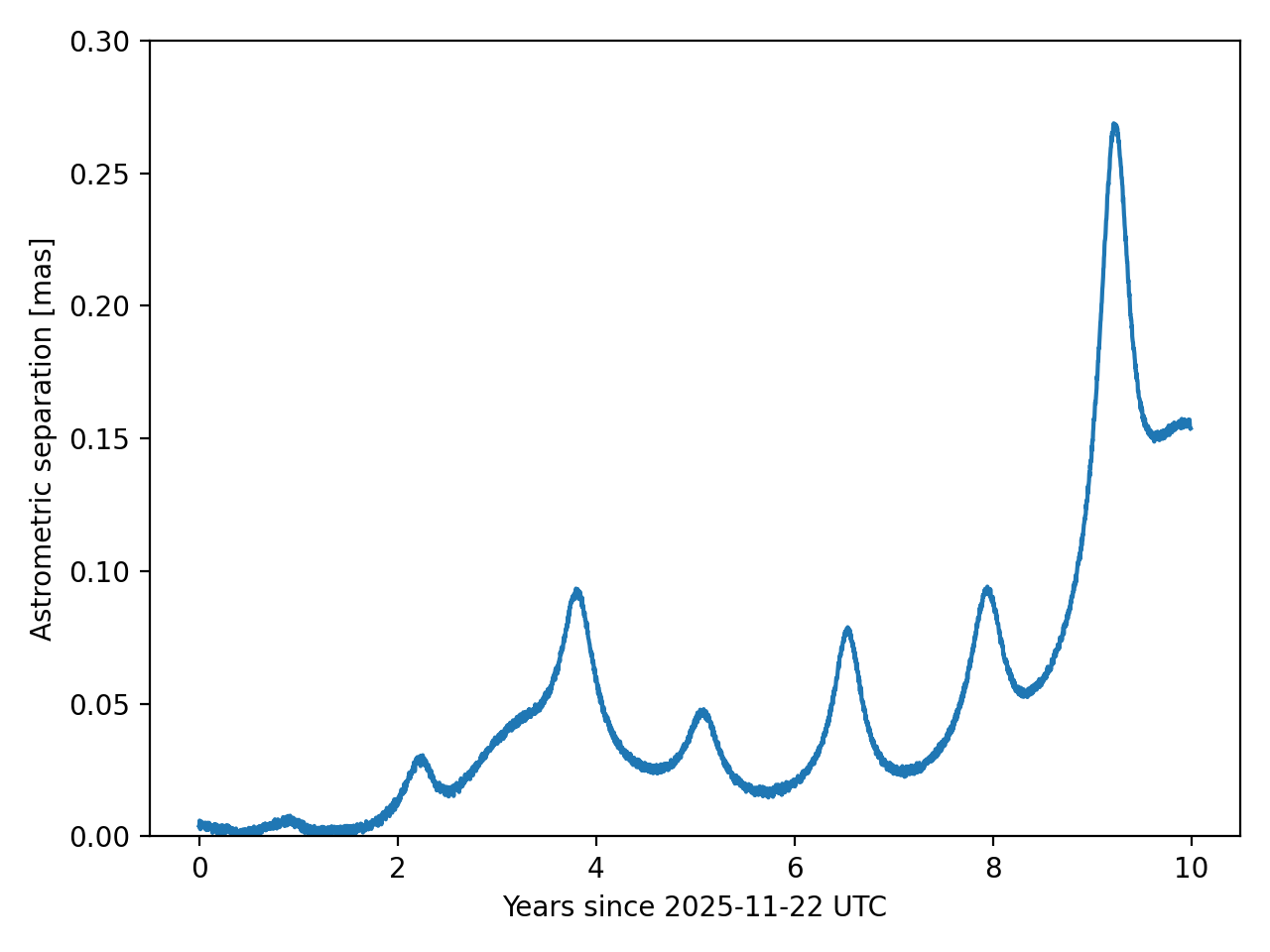
Use the same target, observer, and daily UTC grid in Horizons. Compare DiffOrb astrometric RA and DEC with Horizons RA and DEC.

import astropy.units as u
import numpy as np
from astropy.coordinates import SkyCoord
from astroquery.jplhorizons import Horizons

t_horizons = t_obs_start + jnp.arange(0.0, 3650.0, 1.0)
optical_daily = generator.optical_table(t_horizons, observer)
epochs_utc_jd = np.asarray(t_horizons.utc.jd, dtype=float)

horizons = Horizons(
    id="85472",
    location="327",
    epochs={"start": "2025-11-22", "stop": "2035-11-19", "step": "1d"},
)
eph = horizons.ephemerides(
    refsystem="ICRF",
    refraction=False,
    extra_precision=True,
    cache=False,
)

difforb_astrometric = SkyCoord(
    ra=np.asarray(optical_daily.astrometric_ra, dtype=float) * u.deg,
    dec=np.asarray(optical_daily.astrometric_dec, dtype=float) * u.deg,
    frame="icrs",
)
horizons_astrometric = SkyCoord(
    ra=np.asarray(eph["RA"], dtype=float) * u.deg,
    dec=np.asarray(eph["DEC"], dtype=float) * u.deg,
    frame="icrs",
)

separation = difforb_astrometric.separation(horizons_astrometric).to(u.mas)
values = separation.value

print("COUNT", len(values))
print(
    "MIN_MAX_MEDIAN_P95",
    float(values.min()),
    float(values.max()),
    float(np.median(values)),
    float(np.percentile(values, 95)),
)
print("FIRST3", values[:3])
print("HORIZONS0", float(eph["RA"][0]), float(eph["DEC"][0]))

Output

COUNT 3650
MIN_MAX_MEDIAN_P95 0.0002265390586468172 0.2688633196678126 0.03117657213906492 0.15746311558315265
FIRST3 [0.00397177 0.00392566 0.00597746]
HORIZONS0 299.630791546 -12.72869935

The separation is in milliarcseconds. In this run, it stays below 0.3 mas over 3650 daily epochs.

import matplotlib.pyplot as plt

years = (epochs_utc_jd - epochs_utc_jd[0]) / 365.25

fig, ax = plt.subplots()
ax.plot(years, separation.value)
ax.set(
    xlabel="Years since 2025-11-22 UTC",
    ylabel="Astrometric separation [mas]",
)
ax.set_ylim(0.0, 0.3)

Compare 100 Numbered Small Bodies

This check draws 100 numbered small bodies with a fixed seed, queries one Horizons BCRS Cartesian state for each body at the same initial epoch, propagates the whole batch in DiffOrb, and compares the astrometric optical output with Horizons.

Use one fixed TDB initial epoch for all target states. Use one fixed UTC grid for the observer ephemerides. The observer is Xinglong Station (327). The target sample below uses the numbered-asteroid range stored with this validation run. If the numbered-asteroid range is refreshed from JPL SBDB, the selected target IDs can change.

from pathlib import Path

import astropy.units as u
import matplotlib.pyplot as plt
import jax.numpy as jnp
import numpy as np
from astropy.coordinates import SkyCoord
from astroquery.jplhorizons import Horizons
from tqdm import tqdm

from difforb.body import Site, SmallBody
from difforb.core import BCRS, State, Time

target_count = 100
random_seed = 43
number_min = 1
number_max = 895_910
excluded_target_ids = {
    1, 2, 3, 4, 7, 10, 15, 16, 31, 52, 65, 87, 88, 107, 511, 704
}

initial_epoch = Time.from_tdb_date(2026, 1, 1)
initial_epoch_jd = float(np.asarray(initial_epoch.tdb().jd))

time_offsets = np.arange(0.0, 365.0 * 10.0, 10.0)
compare_times = Time.from_utc_date(2026, 1, 1) + jnp.asarray(time_offsets)
horizons_range = {
    "start": "2026-01-01",
    "stop": "2035-12-22",
    "step": "10d",
}

rng = np.random.default_rng(random_seed)
selected = set()
while len(selected) < target_count:
    target_id = int(rng.integers(number_min, number_max + 1))
    if target_id in excluded_target_ids:
        continue
    selected.add(target_id)

target_ids = np.array(sorted(selected), dtype=int)
observer_code = "327"
observer = Site.from_code(observer_code).require_ground()

Fetch one Horizons BCRS Cartesian state at the same TDB epoch for each target.

def fetch_bcrs_state(target_id):
    table = Horizons(
        id=str(target_id),
        id_type="smallbody",
        location="@0",
        epochs=initial_epoch_jd,
    ).vectors(
        refplane="frame",
        aberrations="geometric",
        cache=True,
    )
    row = table[0]
    return {
        "target_id": int(target_id),
        "x": float(row["x"]),
        "y": float(row["y"]),
        "z": float(row["z"]),
        "vx": float(row["vx"]),
        "vy": float(row["vy"]),
        "vz": float(row["vz"]),
    }


state_rows = []
for target_id in tqdm(target_ids):
    state_rows.append(fetch_bcrs_state(target_id))

initial_epoch_floor = np.floor(initial_epoch_jd)
state_epoch = Time.from_tdb_jd(
    np.full(len(state_rows), initial_epoch_floor),
    np.full(len(state_rows), initial_epoch_jd - initial_epoch_floor),
)

initial_state = State(
    tdb=state_epoch.tdb(),
    pos=np.column_stack(
        [
            [row["x"] for row in state_rows],
            [row["y"] for row in state_rows],
            [row["z"] for row in state_rows],
        ]
    ),
    vel=np.column_stack(
        [
            [row["vx"] for row in state_rows],
            [row["vy"] for row in state_rows],
            [row["vz"] for row in state_rows],
        ]
    ),
    frame=BCRS,
)

Create one batched SmallBody, propagate it for the full comparison interval, and build one batched optical table. Start the stored trajectory before the first observer epoch so the light-time solve stays inside the propagated interval. The grid=True call returns one time series for each target.

target_batch = SmallBody.create(initial_state)
target_batch = target_batch.propagate(
    t_start=Time.from_utc_date(2025, 12, 20).tdb(),
    t_end=Time.from_utc_date(2036, 1, 3).tdb(),
    force_model=force_model,
    integrator=integrator,
)

batch_generator = EphemerisGenerator(target_batch)
difforb_optical = batch_generator.optical_table(
    compare_times,
    observer,
    grid=True,
)

difforb_coord = SkyCoord(
    ra=np.asarray(difforb_optical.astrometric_ra, dtype=float) * u.deg,
    dec=np.asarray(difforb_optical.astrometric_dec, dtype=float) * u.deg,
    frame="icrs",
)

Query Horizons for the same objects, observer, and UTC grid. id_type="smallbody" keeps numbered small bodies separate from major-body IDs.

horizons_ra = np.empty((len(target_ids), len(time_offsets)))
horizons_dec = np.empty_like(horizons_ra)

for row_index, target_id in enumerate(tqdm(target_ids)):
    eph = Horizons(
        id=str(target_id),
        id_type="smallbody",
        location=observer_code,
        epochs=horizons_range,
    ).ephemerides(
        refsystem="ICRF",
        refraction=False,
        extra_precision=True,
        quantities="1",
        cache=True,
    )
    if len(eph) != len(time_offsets):
        raise RuntimeError(f"{target_id} returned {len(eph)} epochs")

    horizons_ra[row_index] = np.asarray(eph["RA"], dtype=float)
    horizons_dec[row_index] = np.asarray(eph["DEC"], dtype=float)

horizons_coord = SkyCoord(
    ra=horizons_ra * u.deg,
    dec=horizons_dec * u.deg,
    frame="icrs",
)

separation = difforb_coord.separation(horizons_coord).to_value(u.mas)

print("TARGETS", len(target_ids))
print("EPOCHS", len(time_offsets))
print("MEDIAN_MAS", float(np.median(separation)))
print("P95_MAS", float(np.percentile(separation, 95)))
print("P99_MAS", float(np.percentile(separation, 99)))
print("MAX_MAS", float(np.max(separation)))

Output

TARGETS 100
EPOCHS 365
MEDIAN_MAS 0.03903224717521309
P95_MAS 0.2738868930459874
P99_MAS 0.48034178172244024
MAX_MAS 1.0784751105453636

Plot the epoch-wise percentile envelope and the cumulative distribution of all separations. The full run makes 100 x 365 comparisons.

years = np.asarray(time_offsets, dtype=float) / 365.25
p00, p05, p50, p95, p100 = np.percentile(separation, [0, 5, 50, 95, 100], axis=0)
flat = np.sort(separation.ravel())
cdf = np.arange(1, flat.size + 1, dtype=float) / flat.size

fig, (ax_time, ax_cdf) = plt.subplots(1, 2, figsize=(6.85, 2.85))

ax_time.fill_between(years, p00, p100, color="0.55", alpha=0.12, linewidth=0, label="0-100 percentile")
ax_time.fill_between(years, p05, p95, color="#1f77b4", alpha=0.18, linewidth=0, label="5-95 percentile")
ax_time.plot(years, p50, color="#1f77b4", linewidth=1.6, label="median")
ax_time.axhline(1.0, color="0.25", linestyle=(0, (4, 3)), linewidth=0.9, label="1 mas")
ax_time.set_yscale("log")
ax_time.set_xlabel("propagation time [yr]")
ax_time.set_ylabel("DiffOrb-Horizons separation [mas]")
ax_time.legend()

ax_cdf.plot(flat, cdf, color="0.4", linewidth=1.5)
ax_cdf.axvline(np.median(separation), color="#1f77b4", linewidth=1.1, label="median")
ax_cdf.axvline(np.percentile(separation, 95), color="#d95f02", linewidth=1.1, label="95th")
ax_cdf.axvline(1.0, color="0.25", linestyle=(0, (4, 3)), linewidth=0.9, label="1 mas")
ax_cdf.set_xscale("log")
ax_cdf.set_xlabel("DiffOrb-Horizons separation [mas]")
ax_cdf.set_ylabel("cumulative fraction")
ax_cdf.legend()

fig.tight_layout()

fig_path = Path("numbered-small-bodies-vs-horizons.png")
fig.savefig(fig_path, dpi=400)
print(fig_path)

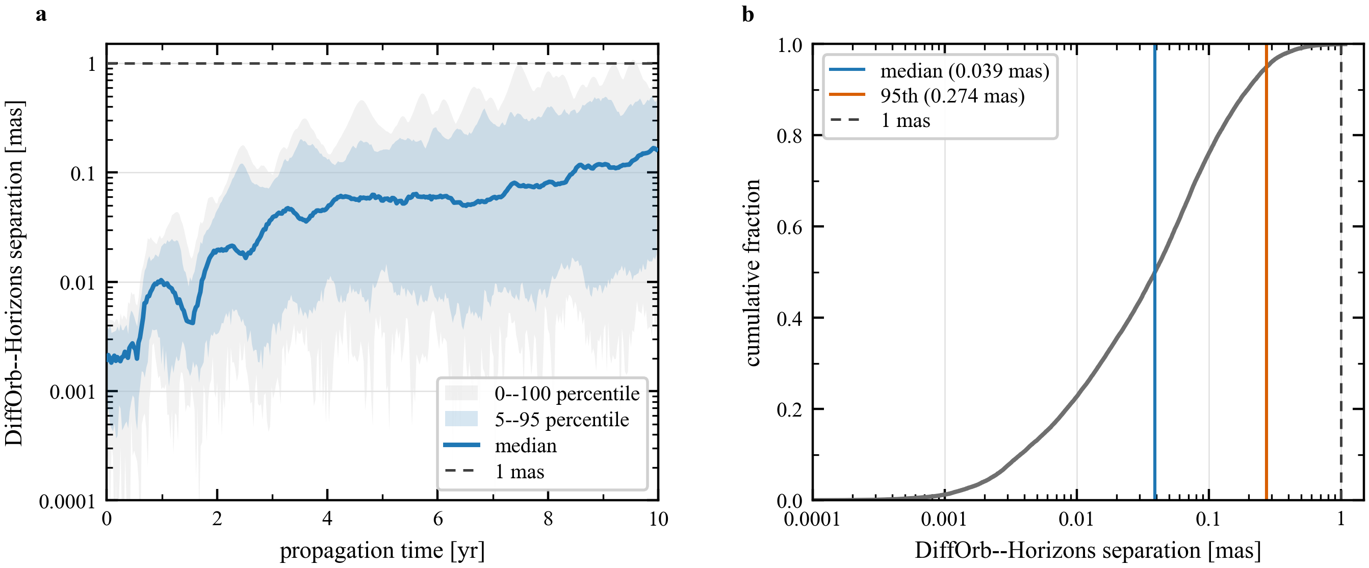
This batch comparison is a broad external check. It is not a fixed acceptance test. The result can change when Horizons updates an orbit solution, when the random sample changes, or when a different force model, observer, kernel set, or numbered-asteroid range is used.

Result

This workflow produces these products from one propagated SmallBody:

• an optical table
• a vector table
• a radar prediction
• an element table
• apside and close-approach event tables
• a Horizons comparison for optical astrometry
• a 100-target Horizons comparison plot for numbered small bodies

The numeric output above used DE441, SB441-N16, Xinglong Station (327), and a fixed random sample of numbered small bodies. Small numerical differences can appear across platforms, JAX or XLA versions, dependency versions, and Horizons service revisions.